Example 3: Curves of Cubic Equations
To generate data curves for cubic equations in the form of
![]()
we construct a computation flow diagram as following:
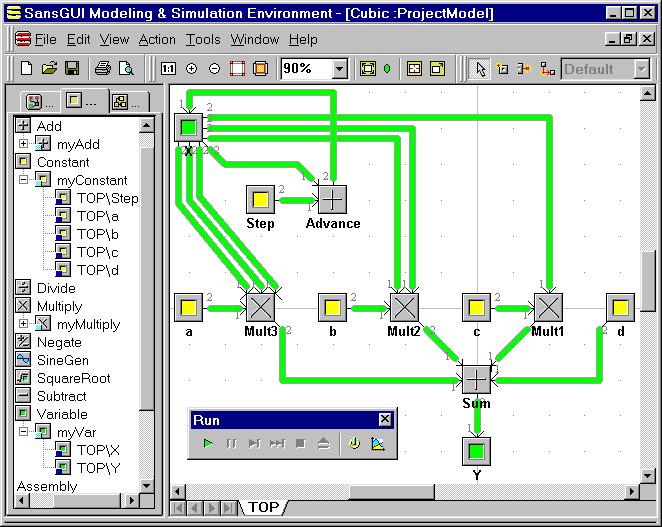
The inputs to Mult3 have a constant a and three links from variable X, meaning that the value in X will be used three times to yield the cubic power of X. At Mult2, there are two links from X and one from variable b for the second order term in the equation. Mult1 calculates c times X, which is pretty straight forward. All these results are summed up with the value of d to obtain the final value of Y. A loop in the flow diagram is formed by the parts: X, Step, and Advance. It is used to walk through a range of X values in order to calculate the Y values. The cycling is controlled by the parameters set in the simulation control object in the Project Model. Please see below for more details.
The Default simulation control object can be found in the Tree View of the Object tab (the first tab) in the Left Pane. It is under the SimCtrl.Cycle.Calc_Default path. Double clicking on the name Default or its icon will pop up the following Object Properties dialog:
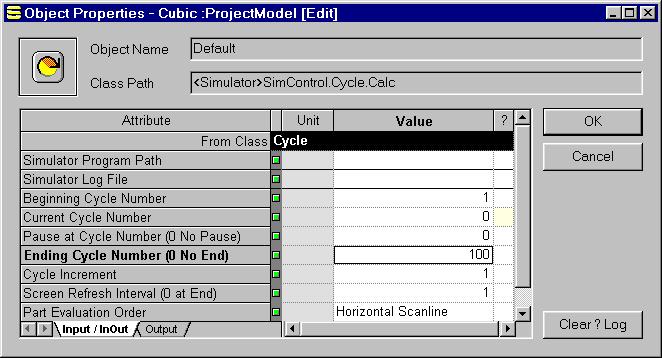
The first field, Simulator Program Path, specifies where the simulator's DLL executable is located. If SansGUI displays an error message about not being able to find the executable, you can right click on this field, select Input Assistant from the context menu and then click on the <File/Dir>... button to find the Visual Calculator's DLL file. The other field of concern is the Ending Cycle Number. It is set to cycle through all parts 100 times in this case. You can set it to a different value if needed. The number of cycles specified here in conjunction with the value set in the Step part and the initial value of X, decide the range of X the simulation will go through. In the example with 100 cycles, the Step value is set to 0.1 and the initial X value is set to -5; therefore, the simulation will go from -5.0 to +4.9 (-5.0 is used in cycle number 1) with 0.1 increments. The Part Evaluation Order is set to the Horizontal Scanline, going from top down.
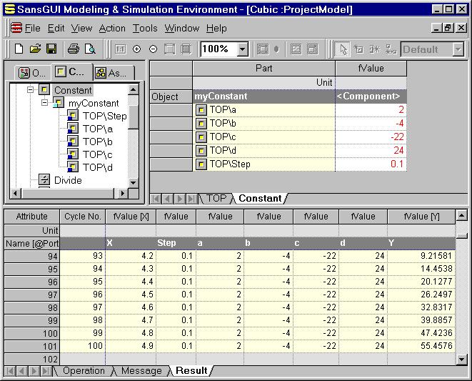
The results of the simulation are logged in the Result View in the Bottom Pane. As shown in the following figure, the X column is marked fValue [X] in the header and the Y column is marked fValue [Y]. They are selected as the x and y data, respectively, for plotting purposes. You can change the plotting selections by right clicking on the data columns and select/unselect the data. However, it would not be interesting in this example because data in all other columns stay constant.
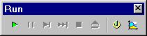
Starting from SansGUI version 1.1, you don't need to pause a simulation or wait until it ends to plot the results. You can click on the Plot Results button, shown as the right-most button in the Run toolbar above, at any time. When the Plot Results dialog is displayed during a simulation run, its contents will be updated at each screen refresh cycle. You are encouraged to experiment this new feature to see the data curve being dynamically updated.
To get the X-Y plot, simply click on the Plot Results button in the Run toolbar. A chart similar to the following will be shown (after a simulation run, the horizontal grid lines are added via the Grid Lines>Y Axis selection from the right click context menu):
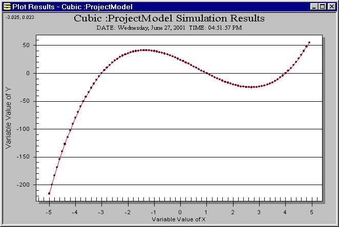
The coordinates in at the upper-left corner will be updated as you move your mouse pointer in the charting area. You can move the mouse pointer to the near 0 value of Y along the data curve to see what the roots of X should be in the equation. You can also use the right-click context menu to customize the chart.
If SansGUI cannot find the simulator DLL, please consult the instructions on Setting Simulator DLL Location at the bottom of Example 1.
As an exercise, change the values of a, b, c, and d to see how the new curves will be constructed. You may have to adjust the X ranges to see the curves being plotted in more appropriate scales. If you continue to click on the Run In-Process button without hitting the Reset Data button, the starting value of X will be its ending value of the previous run. You can also set up a scrolling frame for the simulation run:
Select Tools>Options... from the pull-down menu.
Change Maximum Number of Rows in the Result Views to 50 (the default is 1000).
Click on the OK button to commit the change.
Open the Properties dialog of the Default simulation control object. If you have forgotten how to do it, please see the Controlling Cycles section above.
Change the Ending Cycle Number (0 No End) to 0, indicating that we want to continuously run the simulation.
Click on the OK button to save the change.
Click on the Reset Data button in the Run toolbar.
If the Plot Results dialog is not displayed, click on the Plot Results button to pop it up.
Click on the Run In-Process button to start the simulation.
You can see a range of X being displayed in the chart and the plot frame being scrolled to the right as the simulation continues. At this moment, you can click on the Pause button in the Run toolbar to pause the simulation, or click on the Stop button to terminate the simulation. When the simulation is paused, you can click on the Step button to advance the simulation one cycle at a time.
Visual Calculator for SansGUI Version 1.1
Copyright © 2001-2003 ProtoDesign, Inc. All rights reserved.