|
| |
Application Programs for SansGUI
The following programs demonstrate scientific and engineering applications
using the SansGUI Modeling and Simulation Environment.
Some of the programs are available for testing, and they may
include source code for educational purposes. Please check the
descriptions of each program for details.
-
Mixer - Solving a System of Linear
Equations: demonstrates how to programmatically prepare necessary
matrices and tables for a chemical reactor/mixer network with various
concentrations and flow rates in the components, a typical engineering
problem that involves a system of linear equations. The equations are solved by using Naive Gauss Elimination or LU Decomposition
algorithms, or calling the MATLAB engine from The Mathworks, Inc.
Mixer -- Solving a System of Linear Equations
-
Description
Project Mixer is a programming example that
demonstrates how a simulator can be developed to solve a system of linear
equations in a typical engineering application, using the SansGUI Modeling
and Simulation Environment. A mixer is a chemical reactor that takes a
mixture from a number of input sources with various concentrations and flow
rates and produces a homogeneous mixture with a new concentration. It
can be connected to other mixers, sources or sinks with in-flow and out-flow
pipes. Applying the law of mass conservation, this example shows how
to set up and load a constant matrix and provide a table for the right hand
side constants of the equations as well as a data column for the solutions.
A second matrix is created to store the inverse matrix for further
analyses. The sizes of the matrices and the table are set through the
program according to the number of mixers in a project
model created by the user in the SansGUI Run-Time environment. The
user can select one of the three solution methods before a simulation run:
1) Naive Gauss Elimination, 2) LU Decomposition, or 3) Call MATLAB
Engine. The first two selections use the corresponding algorithms
implemented in the simulator. When 3) Call MATLAB Engine is chosen,
the user needs to have the MATLAB software installed in his/her
machine. MATLAB can be obtained from The MathWorks, Inc. Independent
implementations of the project written in Microsoft Visual C/C++ and Compaq
Visual Fortran are included with full source code.
-
Demonstration
Click on a picture to obtain its full size screen
shot.
|
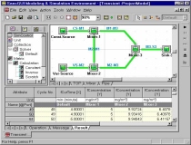 |
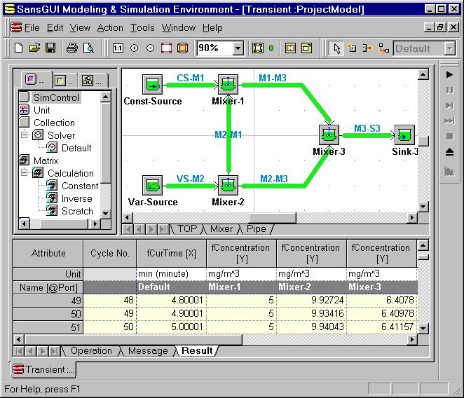
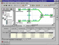
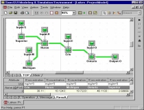
This example model contains three mixers:
Mixer-1 takes a constant source; Mixer-2 takes a variable source; Mixer-3
combines the output of the first two. In this first example, the
pipe from Mixer-2 to Mixer-1 is shut-off, with the flow rate set to 0.
|
|
 |
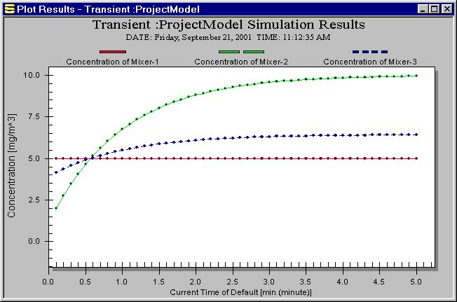
With no in-flow from Mixer-2, Mixer-1 stays
constant. Both Mixer-2 and Mixer-3 have variable concentrations,
affected by the variable source flows into Mixer-2..
|
|
 |
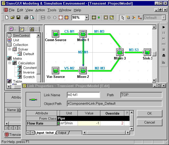
In the second scenario, we "open"
the pipe from Mixer-2 to Mixer-1 by setting the flow rate to 2 m3/min.
The output flow rates of the pipes from Mixer-1 and Mixer-2 to Mixer-3 are
also modified to reflect the change.
|
|
 |
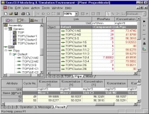
Affected by the incoming flow from Mixer-2
and its variable source, Mixer-1 has its concentration changed through
time in the second scenario. The changing values are shown in the
Result View in the Bottom Pane. |
|
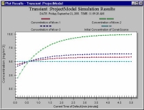 |
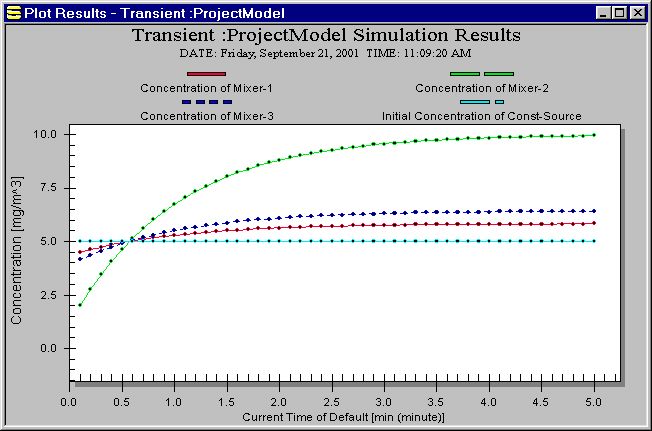
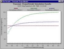
This plot shows Mixer-1 has various
concentrations through time after the pipe from Mixer-2 to Mixer-1 is
opened. |
|
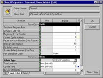 |
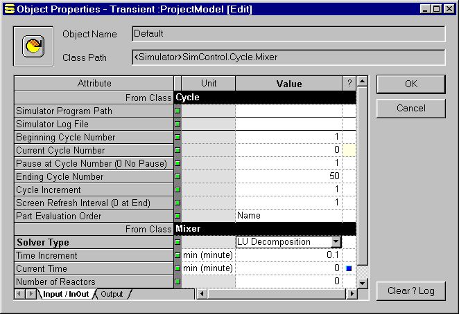
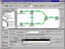
The simulation user can select 1) Naive
Gauss Elimination, 2) LU Decomposition, or 3) Calling MATLAB Engine in the
simulation control object properties. These options are created by
the simulation developers using the SansGUI Development Environment. |
|
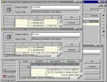 |
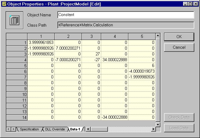
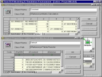
A constant matrix, an inverse matrix, and a
table that stores the right-hand-side (r-h-s) constants and the solution
vector can be examined by the simulation user during and after a
simulation run. Because there are three mixers, the constant matrix
is a 3x3 matrix. |
|
 |
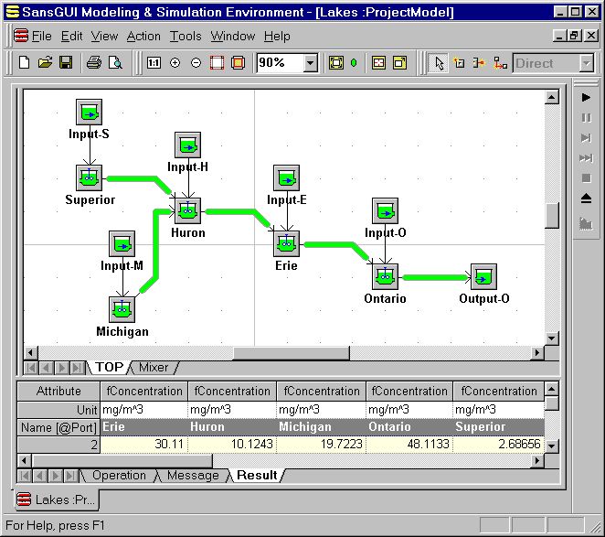
This example shows a model of chloride
concentrations in the Great Lakes, taken from an exercise problem in
Chapra & Canale. The solution is shown in the Result View in the
Bottom Pane. |
|
 |
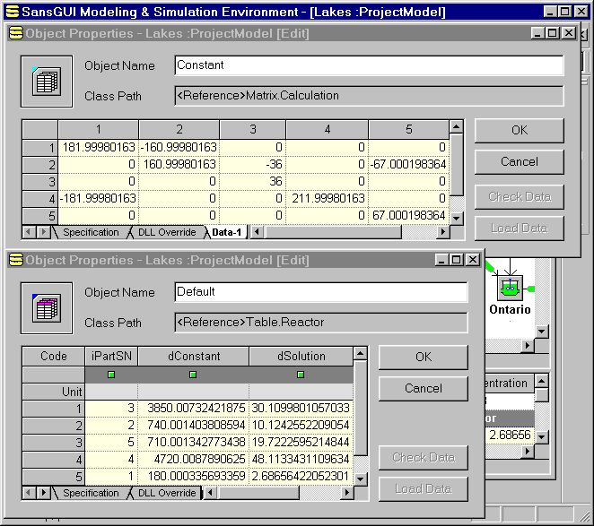
The constant matrix and the table of r-h-s
constants and solutions are examined. These are created
programmatically prior to calling the solution routines. |
|
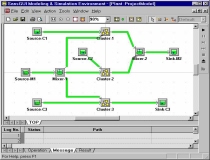 |
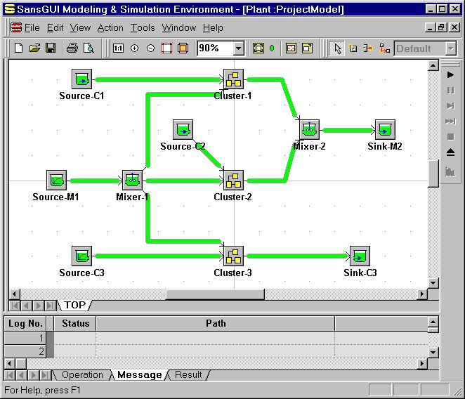
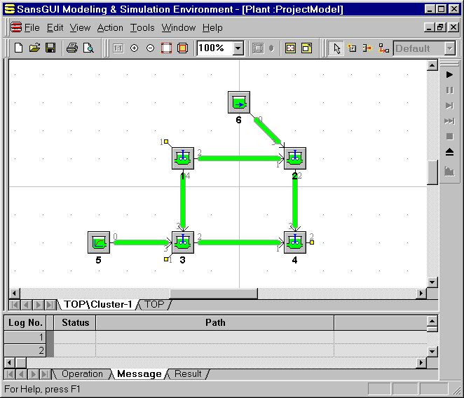
This example shows a more elaborated model
with three nearly identical subassemblies -- Cluster-1 through
Cluster-3. The first cluster was created manually while the second
and the third clusters are replicas of the first one, created by using the
Clone Part facility in SansGUI. |
|
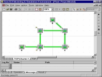 |
Each cluster contains a subassembly
depicted in this figure. Three ports, two input ports and one output
port, are exported from this subassembly for connections in the TOP
assembly level. |
|
 |
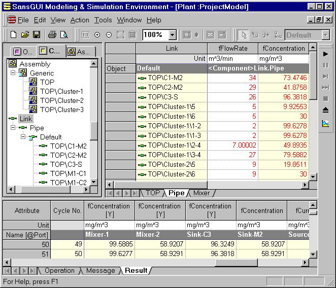
The flow rates of all pipes (the data
column with white background) can be entered in a Grid View in the Right
Pane. Also shown in the Grid View are the calculated concentrations
of all pipes in the protected fields (light yellow background). |
|
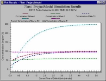 |
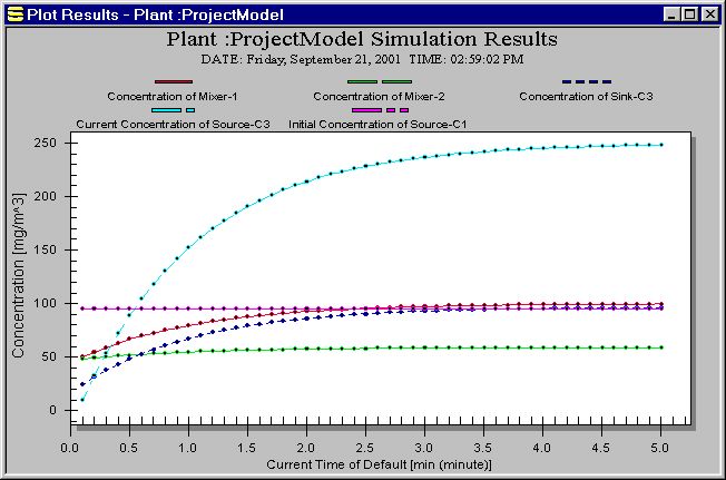
The concentrations of some of the
components through time are plotted. These are selected from the
data columns of the Result View in the previous figure. |
|
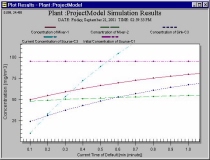 |
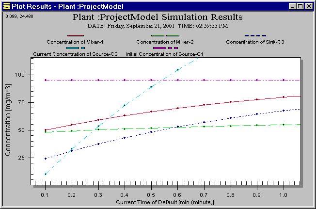
The lower left corner of the previous plot
is zoomed in to study the beginning minute of the simulation in more
detail. The user can select a rectangular area on the plot for multi-level zooming. |
|
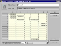 |
The constant matrix of the example with
multiple subassemblies is examined. There are fourteen mixers in
this model, yielding a 14x14 matrix. |
-
Detail
A typical engineering problem
involves a network of system components that can be modeled mathematically
with a set of linear equations established with certain physical laws.
The unknowns in the equations represent the properties that the engineer
would like to investigate, given a set of known conditions. In this
example, we use chemical reactors that mix conservative chemical fluid from
input sources with various concentrations and dispense the new mixture to
other mixers and/or sinks. A pipe used to link two components controls
the flow rate of the mixture that travels from one component to the
other. Normally, the sum of all the input flow rates is equal to the
sum of all the output flow rates in a mixer so that the volume can stay
constant. The concentration in each mixer (assumed to be uniform) are
the unknowns that we would like to solve.
With the SansGUI Modeling and
Simulation Environment, the simulator is implemented in an object-oriented
manner. Using the SansGUI Run-Time Environment, instances of Mixers,
Sources and Sinks can be created and connected with Pipes,
derived from the Link class. The linear equation solver is
implemented in Class Solver, derived from Class Collection.
Three calculation matrices and a reactor table are reference objects used
during the calculation process. We implemented the Naive Gauss
Elimination and LU Decomposition algorithms in C/C++ and Fortran
independently. Both C/C++ and Fortran implementation of the MATLAB
engine calls are also provided to demonstrate how SansGUI can be used in
conjunction with MATLAB.
-
Code
The implementation of this example can be found in
the functions of seven classes: Base.Container.Reactor, Base.Container.Sink,
Base.Source, Base.Source.Variable, Collection.Solver, Matrix.Calculation, and
Table.Reactor. Click on the following links to see all the necessary code for this
project. The C/C++ and Fortran implementations are independent; only
one of them is required.
-
Download
The entire project, including the program with its
source code, on-line documentation, and the examples are available from our Download
page. This project requires the SansGUI Modeling and Simulation
Environment. A demonstration version of SansGUI (SGdemo) can be
obtained from the same Download page.
-
Reference
-
Chapra, Steven C. & Canale, Raymond
P. 1998. Numerical Methods for Engineers: with
Programming and software Applications, 3rd Ed., WCB/McGraw-Hill, Boston,
Massachusetts.
-
The Mathworks, Inc. 1998. MATLAB
Application Programming Interface Guide, Version 5.0. Natick,
Massachusetts. An External
Interfaces/API Manual can be accessed on-line via The Mathworks' web
site.
-
ProtoDesign, Inc. 2001. SansGUI
Version 1.0 Document Set, Bolingbrook, Illinois. The whole set of SansGUI
Manuals can be accessed on-line.
-
Credit
This example is developed by the SansGUI
Development Team at ProtoDesign, Inc. The Great Lakes example is taken
from Exercise 12.7 of Chapra & Canale. The Fortran and C
implementations of Naive Gauss Elimination and LU Decomposition use the
algorithms introduced in Chapra & Canale's text. MATLAB is a
registered trademark of The Mathworks, Inc.
|